This tutorial will take users through the process of peak calling with Q and will demonstrate a number of typical steps in the downstream analysis. If you have not yet downloaded Q, please see the section on installation before going further.
This tutorial is subdivided into the following sections:
Q requires as input a file representing the aligned ChIP-seq read data in BAM or SAM format. If the ChIP-seq experiment was performed with a generic IgG control (as is to be recommended), there will be one BAM/SAM file for the experiment with the specific antibody ("treatment") and one BAM/SAM file for the experiment with generic IgG ("control"). If you are starting with unmapped FASTQ files, alignment can be performed with a number of programs including bwa and bowtie. In general, it is recommended that reads that map to multiple positions in the genome (i.e., repetitive sequences) should be removed prior to ChIP-seq analysis (For instance, non-uniquely mapped reads are tagged with 'XT:A:U' by bwa for single end data, and can be removed by bowtie using the options '--best -m 1'). For the purposes of this tutorial, we will use aligned ChIP-seq reads from the ENCODE project, it is also possible to download the corresponding BAM files via web browser from UCSC. Alternatively, the same BAM files can be downloaded using wget.
wget -N ftp://hgdownload.cse.ucsc.edu/goldenPath/hg19/encodeDCC/wgEncodeHaibTfbs/wgEncodeHaibTfbsHct116Pol24h8V0416101AlnRep*;According to the ENCODE guidelines for ChIP-seq, experiments should be accompanied by control experiments. At the UCSC ENCODE browser, you can find the contol dataset that corresponds to a given experiment by looking for the controlId in the Additional Details section. For instance, for one experiment we find controlId=SL3457; in the Additional Details section. In order to find the corresponding control experiment, search for 'Lab provided indentifier' is among 'SL3457'. Again, the BAM files may be downloaded via web browser or wget.
wget -N ftp://hgdownload.cse.ucsc.edu/goldenPath/hg19/encodeDCC/wgEncodeHaibTfbs/wgEncodeHaibTfbsHct116RxlchV0416101AlnRep1.*;In this case, this will leave you with six files, two BAM files for the replicates and one for the control, as well as the three corresponding BAM index files. If desired, the mapped ChIP-seq data can now be directly visualized using the Integrative Genome Viewer.
Q can be applied directly to the downloaded datasets. Due to Q's statistical model there is no need for downsampling of control data. It is generally recommended to remove duplicates (i.e. multiple reads mapping to the same position) before peak calling. Duplicate reads can originate from PCR errors during library preparation, Q removes duplicates on the fly (without altering the original BAM file), thus obviating the need for using a separate program such as samtools to remove duplicate reads. If you have already removed duplicate reads, no additional adjustments are required for Q. Note that Q allows multithreading. In order to use n threads to perform the analysis, pass the argument '--thread-num n' to the command line (e.g., '--thread-num 8' for 8 threads). If you want to print additional progress information to the screen use the option '--verbose'. The option '--help' will show information about all command line arguments. To perform the basic analysis, you need to indicate the path to the treatment dataset (with the '-t' flag) and the name of the prefix you want for the output files of Q (with the '--out-prefix' flag). If a control experiment was performed, the path to the corresponding BAM file is indicated with the '-c' flag.
In the following example, we perform peak calling on replicate 1 and 2 for a ChIP-seq experiment involving RNA polymerase II in HCT-116 cells (GSM803474). The file names of the corresponding BAM files are those from the UCSC ENCODE ChIP-seq browser. The command assumes that the treatment and control BAM files are located in the current working directory.
Q -t wgEncodeHaibTfbsHct116Pol24h8V0416101AlnRep1.bam -c wgEncodeHaibTfbsHct116RxlchV0416101AlnRep1.bam -o Hct116Pol24h8Rep1 -wbt -wbcQ -t wgEncodeHaibTfbsHct116Pol24h8V0416101AlnRep2.bam -c wgEncodeHaibTfbsHct116RxlchV0416101AlnRep1.bam -o Hct116Pol24h8Rep2 -wbtThe additional flags '-wbt' and '-wtc' cause the generation of bedGraph files for treatment and control (see below).
After the analysis is finished, you will find the following files for replicate 1 (and analogous files for replicate 2).
| Filename | Description |
|---|---|
| Hct116Pol24h8Rep1-Q-runinfo.txt | Contains all chosen parameters and general information about the run. |
| Hct116Pol24h8Rep1-Q-binding-characteristics.R | R script that generates a plot for the fragment-length estimation procedure. |
| Hct116Pol24h8Rep1-Q-quality-statistics.tab | Contains useful quality statistics regarding the performance of the corresponding ChIP-seq experiment. |
| Hct116Pol24h8Rep1-Q-narrowPeak.bed | The actual result and contains the predicted binding sites. Find a detailed description of the narrowPeak format here. |
| Hct116Pol24h8Rep1-Q-treatment.bedgraph | Contains signal density profile for treatment data which can be loaded as custom track within genome browser of UCSC. Find a detailed description of the bedGraph format here. |
| Hct116Pol24h8Rep1-Q-control.bedgraph | Contains signal density profile for the control data. |
Q outputs an R script that allows users to visualize the results of the fragment-length estimation procedure (similar to the "binding characteristics analysis" of SPP). This file can be used to generate a graphic in R. In our example, the file Hct116Pol24h8Rep1-Q-binding-characteristics.R is used to generate the the corresponding plot Hct116Pol24h8Rep1-Q-binding-characteristics.pdf by entering the following command in the shell:
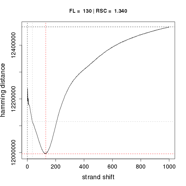
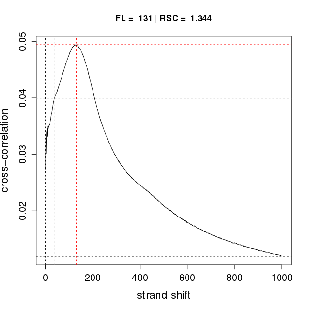
Rscript Hct116Pol24h8Rep1-Q-binding-characteristics.RThe pdf file for replicate 1 is shown below on the left. If SPP is applied to the same dataset (following duplicate removal by samtools), an analogous, but vertically flipped curve with nearly identical characteristics is generated, shown on the right.


Binding characteristics plot for Hct116Pol2Rep1 for Q (left) and SPP (right)
The main difference is that Q calculates the Hamming distance, whereas SPP calculates the Pearson correlation coefficient. The shift with the minimum Hamming distance is taken as the estimate of the average fragment length by Q, while the shift with the maximum correlation is taken as the estimate of the average fragment length by SPP. The RSC values reflect quality of enrichment and are used as a quality metric for ENCODE data, are almost identical for Q and SPP. The RSC value is a useful metric for trouble shooting and optimization ChIP-seq protocols. We compared the results of the binding characteristics analysis on 38 datasets, and found comparable estimates of fragment length and RSC for Q and SPP.
Q provides you with feedback about the performance of your ChIP-seq experiment. This is useful for trouble-shooting and enables you to evaluate the quality of your data relative to many published datasets from ENCODE. The number of uniquely mapped non redundant reads or hits (UMNRH) that actually map to real binding sites of the probed factor is a good measure for the overall performance of your ChIP-seq experiment, the more the better. This number depends roughly on three factors, the number of uniquely mapped reads, the complexity of your sequencing library and the efficiency of the enrichment. Q provides you with quality metrics for all of these factors.
The complexity of the library is reflected by the duplication rate, which is given as the proportion of uniquely mapped reads that are redundant, i.e. there are at least two reads having identical sequences. Redundant reads can originate from PCR errors during library preparation. A high duplication rate means a low complexity of the library.
The efficiency of enrichment is measured as the Q's enrichment score (QES). This is a number between 0 and 1, which reflects the efficiency of the IP step and can be interpreted like a signal-to-noise-ratio. A QES of 1 means that all UMNRH occur at binding positions of the probed factor, whereas a QES of 0 means the opposite. The QES is determined by first determining the observed fraction of all UMNRHs in qfrags and then subtracting the expected fraction, where a UMNRH on the forward strand forms a qfrag with a UMNRH on the reverse strand if the distance is at least one estimated fragment length minus 50 and at most one estimated fragment length plus 50.
The duplication rate and the degree of enrichment defines what proportion of the sequenced reads read will appear at binding positions. These two factors are combined in an score, called Q's sample score (QSS). It is defined as 1 minus the duplication rate multiplied with the QES. As the name implies, this is a quality metric for the sample. By multiplying the number of uniquely mapped reads with the QSS the absolute number of hits in signals (ENSH) is estimated.
The tab separated file Hct116Pol24h8Rep1-Q-quality-statistics.tab contains global information for each individual chromosome and for the whole genome. Most of the column names are self-explanatory and a detailed description is as follows.
| Column | Description |
|---|---|
| 1 | Chromosome name |
| 2 | Total number of mapped treatment reads that were used by Q |
| 3 | Number of duplicates that were removed from treatment data |
| 4 | Duplication rate for treatment data |
| 5 | Total number of mapped control reads that were used by Q |
| 6 | Number of duplicates that were removed from control data |
| 7 | Duplication rate for control data |
| 8 | Expected number of hits in qfrags |
| 9 | Observed number of hits in qfrags |
| 10 | Q's enrichment score (QES) |
| 11 | Q's sample score (QSS) |
| 12 | Estimated number of hits in signals (ENSH) |
| 13 | Estimated fragment length |
| 14 | Relative Strand Cross-correlation coefficient (RSC) |
The lines for the individual chromosomes are given for completeness and the most important line is the last one in which the results for the whole genome are summarized. In the first column this line contains the prefix for output given via the option '--out-prefix' and not the chromosome name. This is useful when collecting the results from multiple ChIP-seq experiment in one table. In order to provide you with reference values for the quality metrics introduced above, we analysed 392 datasets from ENCODE. The results are summarized in the table below.
| very low | moderate low | moderate high | very high | |
|---|---|---|---|---|
| UMNRH | <= 11,520,000 | 11,520,000 < | 16,380,000 < | 22,770,000 < |
| DR | <= 0.07 | 0.07 < | 0.13 < | 0.23 < |
| QES | <= 0.13 | 0.13 < | 0.20 < | 0.28 < |
| QSS | <= 0.12 | 0.12 < | 0.16 < | 0.21 < |
| ENSH | <= 2,267,000 | 2,267,000 < | 3,041,000 < | 4,326,000 < |
Use Q with the option '-wbt' and '-wbc' to generate BedGraph files for the fragment coverage profile on the fly. The fragment coverage profile is a popular and intuitive representation of ChIP-seq data. BedGraph (and also BigWig) formated files can be loaded as custom track in UCSC's genome browser, which allows you to present your own data in the context of other related data, for example ChIP-seq data histone modifications or cofactors or expression data. Once you have composed a collection of tracks and found an interesting region you can easily export vector graphics in ps or pdf format, which are especially suited for publication. See the following figure for an illustrative example.

Example for a figure generated in the UCSC genome browser. The upper two tracks display the bigWig files generated in the course of this tutorial. In both replicates analyzed, RNA Pol2 binds to the Notch2 promoter in HTC116 cells. The publicly available ChIP-seq tracks for chromatin marks and RNA-seq in HCT116 cells show that the promoter is active (H3K4me3 (lower green track) and H3K27ac (magenta)) and that the Notch2 gene is transcribed (black track). Also, the dark red track, a ChIP-seq for the transcription factor SRF, shows that SRF binds to the first intron and the corresponding binding site shows H3K4me1 (upper green track) and H3K27ac (magenta) marks typical for active enhancers.
For large datasets the BigWig format is more suitable, because it allows smoother browsing. It is possible to deposit BigWig files on a web accessible server and provide UCSC's genome browser with a link to the data. If you do not have your own web-server, it is also possible to upload bigWig files to an online file storage provider, such as Dropbox*. The next steps will guide you through the generation of BigWig files, the upload to Dropbox, the integration as custom tracks within UCSC's genome browser, as well as the customization and the export of figures.
We will implement the generation of BigWig files for Q as soon as possible. By then the BedGraph files have to be converted using two command line utilities of UCSC, fetchChromSizes and bedGraphToBigWig. These tools can be downloaded for Linux and Mac. Please see section on installation before going further.
The converter bedGraphToBigWig needs information about the chromosome sizes. Use fetchChromSizes to fetch the proper sizes from UCSC.
fetchChromSizes hg19 > hg19.chrom.sizesNow convert the BedGraph files into BigWig format
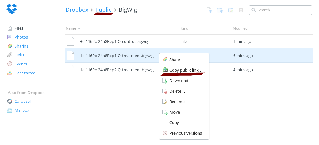
bedGraphToBigWig Hct116Pol24h8Rep1-Q-treatment.bedgraph hg19.chrom.sizes Hct116Pol24h8Rep1-Q-treatment.bigwigbedGraphToBigWig Hct116Pol24h8Rep2-Q-treatment.bedgraph hg19.chrom.sizes Hct116Pol24h8Rep2-Q-treatment.bigwigbedGraphToBigWig Hct116Pol24h8Rep1-Q-control.bedgraph hg19.chrom.sizes Hct116Pol24h8Rep1-Q-control.bigwigNow upload the files to your Dropbox and create public links. It is important to place the files within the public folder, otherwise a public link cannot be created.

Prepare track definition lines for custom tracks in UCSC's genome browser. Use the public links as bigDataUrl. If you generated your own public links edit the text box below correspondingly.
track type=bigWig name="Hct116Pol24h8Rep1" description="Fragment Coverage" visibility=full
 bigDataUrl=https://dl.dropboxusercontent.com/u/35942072/BigWig/Hct116Pol24h8Rep1-Q-treatment.bigwig

track type=bigWig name="Hct116Pol24h8Rep2" description="Fragment Coverage" visibility=full
 bigDataUrl=https://dl.dropboxusercontent.com/u/35942072/BigWig/Hct116Pol24h8Rep2-Q-treatment.bigwig

track type=bigWig name="Hct116Pol24h8Control" description="Fragment Coverage" visibility=full
 bigDataUrl=https://dl.dropboxusercontent.com/u/35942072/BigWig/Hct116Pol24h8Rep1-Q-control.bigwig
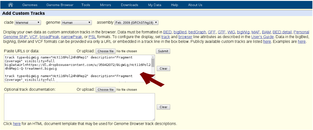
Now go to UCSC's genome browser. After selecting the proper assembly (in our case hg19) select manage custom tracks. On the next page select add custom tracks. Now paste the track definition lines from the text box above into the Paste URLs or data box and select the Submit button.

After a short while you will be back on the manage custom tracks page. Then select go to genome browser where your custom tracks should now be displayed. You can customize each track by right-clicking and selecting configure. Add tracks for related data by selecting track search below the tracks. Export the current browser graphic in pdf or eps format by selesting View at the top and then PDF/PS.